Kolmogorov-Arnold Network with B-Spline approximation

We demonstrate a Kolmogorov-Arnold network whose learned activation functions are B-Spline functions composed with the real.rational input map. This is somewhat similar to the original KAN paper.

import matplotlib.pyplot as plt
import torch
from torch import nn

import torchcurves as tc

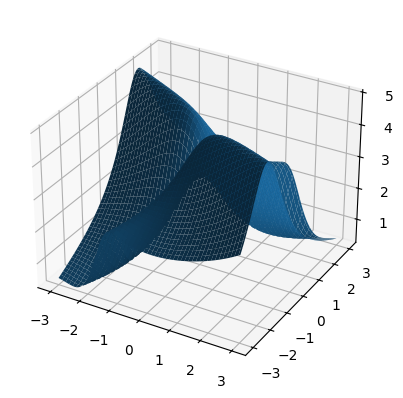
Define regression function

def func(xs):
    pole_1 = torch.tensor(0-2j)
    pole_2 = torch.tensor(0-1j)
    cresult = 10 / (xs[:, 0] + 2 * xs[:, 1] - pole_1) - 2 / (2 * xs[:, 0] - xs[:, 1] - pole_2)
    return cresult.abs()

n = 100
xs = torch.linspace(-3, 3, n)
ys = torch.linspace(-3, 3, n)
grid = torch.cartesian_prod(xs, ys)
zs = func(grid)

ax = plt.figure().add_subplot(projection='3d')
grid_x = grid[:, 0].reshape(n, n)
grid_y = grid[:, 1].reshape(n, n)
plot_z = zs.reshape(n, n)
ax.plot_surface(grid_x, grid_y, plot_z)

<mpl_toolkits.mplot3d.art3d.Poly3DCollection at 0x79ba45bb3560>

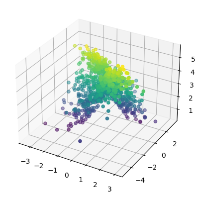
Generate training data

n_samples = 1000
sigma = 0.3
X = torch.randn(n_samples, 2)
y = func(X) + sigma * torch.randn(n_samples)

ax = plt.figure().add_subplot(projection='3d')
ax.scatter3D(X[:, 0], X[:, 1], y, c=y)

<mpl_toolkits.mplot3d.art3d.Path3DCollection at 0x79ba45675700>

Define and train the KAN

input_dim = 2
intermediate_dim = 5
knots = 10

kan = nn.Sequential(
    # layer 1
    tc.BSplineCurve(input_dim, intermediate_dim, knots_config=knots, input_map='real.rational'),
    tc.Sum(dim=-2),
    # layer 2
    tc.BSplineCurve(intermediate_dim, intermediate_dim, knots_config=knots, input_map='real.rational'),
    tc.Sum(dim=-2),
    # layer 3
    tc.BSplineCurve(intermediate_dim, 1, knots_config=knots, input_map='real.rational'),
    tc.Sum(dim=-2),
)

example_data = torch.tensor([[-5, 3], [3, 2], [1, 3]])
output = kan(example_data)
print(output.shape)

torch.Size([3, 1])

n_epochs = 100
batch_size = 32
lr = 5e-3
print_every = 10

dl = torch.utils.data.DataLoader(torch.utils.data.TensorDataset(X, y), batch_size=batch_size, shuffle=True)
optim = torch.optim.Adam(kan.parameters(), lr=lr)
criterion = nn.MSELoss()

for epoch in range(1, 1 + n_epochs):
    epoch_loss = 0.
    for Xb, yb in dl:
        pred = kan(Xb)
        cost = criterion(pred.squeeze(), yb)

        optim.zero_grad()
        cost.backward()
        optim.step()

        epoch_loss += cost * Xb.shape[0]

    epoch_loss /= n_samples
    eval_loss = criterion(kan(grid).squeeze(), func(grid))

    if epoch == n_epochs or epoch % print_every == 0:
        print(f'Epoch {epoch}: train loss = {epoch_loss:.3f}, eval_loss = {eval_loss:.3f}')

/home/alex/git/torchcurves/.venv/lib/python3.12/site-packages/torch/autograd/graph.py:824: UserWarning: CUDA initialization: The NVIDIA driver on your system is too old (found version 11040). Please update your GPU driver by downloading and installing a new version from the URL: http://www.nvidia.com/Download/index.aspx Alternatively, go to: https://pytorch.org to install a PyTorch version that has been compiled with your version of the CUDA driver. (Triggered internally at /pytorch/c10/cuda/CUDAFunctions.cpp:109.)
  return Variable._execution_engine.run_backward(  # Calls into the C++ engine to run the backward pass

Epoch 10: train loss = 0.143, eval_loss = 0.241
Epoch 20: train loss = 0.115, eval_loss = 0.133
Epoch 30: train loss = 0.102, eval_loss = 0.104
Epoch 40: train loss = 0.099, eval_loss = 0.100
Epoch 50: train loss = 0.098, eval_loss = 0.097
Epoch 60: train loss = 0.092, eval_loss = 0.122
Epoch 70: train loss = 0.088, eval_loss = 0.134
Epoch 80: train loss = 0.087, eval_loss = 0.143
Epoch 90: train loss = 0.088, eval_loss = 0.159
Epoch 100: train loss = 0.086, eval_loss = 0.165

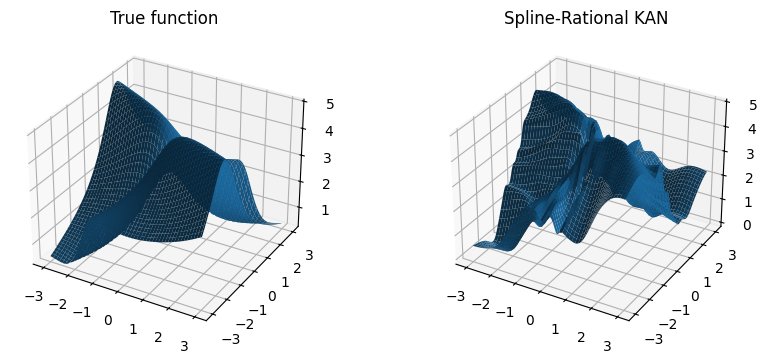
Plot the network and the true function, side by side

with torch.no_grad():
    kan_z = kan(grid).reshape(n, n)

fig = plt.figure(figsize=(10, 4))
ax_left = fig.add_subplot(1, 2, 1, projection='3d')
ax_right = fig.add_subplot(1, 2, 2, projection='3d')

ax_left.set_title('True function')
ax_left.plot_surface(grid_x, grid_y, plot_z)

ax_right.set_title('Spline-Rational KAN')
ax_right.plot_surface(grid_x, grid_y, kan_z)

plt.show()