Legendre curve plotting demo#
In this notebook we show the spectral nature of Legendre curves. The parameters we learn are a kind of a frequency domain, defining the spectrum of the curves. They oscilate more close to the origin, and less farther away from the origin.
[11]:
import matplotlib.pyplot as plt
import torch
import torch.nn.functional as f

import torchcurves.functional as tcf
Define parameters#
[ ]:
degree = 10
n_coefficients = 1 + degree
Define coefficients of various curves#
[66]:
num_curves = 3
dim = 2

t = torch.linspace(-1, 1, n_coefficients)

freq = torch.pi * n_coefficients
first_coef = torch.stack([torch.sin(freq * t), torch.cos(freq * t)], dim=1)
second_coef = torch.stack([torch.sin(freq * t) / f.softplus(t), torch.cos(freq * t) / f.softplus(t)], dim=1)
third_coef = torch.stack([torch.exp(t) / (1 + 5 * (1 + t)), torch.sin(freq * t) / (1 + 10 * (1 + t))], dim=1)
coefs = torch.stack([first_coef, second_coef, third_coef], dim=1)
coefs.shape
[66]:
torch.Size([6, 3, 2])
Sample and draw the Legendre curves with 100 sample points from -1 to 1#
[67]:
sample_points = torch.torch.linspace(-1, 1, 1000)
curve_args = sample_points.reshape(-1, 1).expand(-1, 3)
[68]:
curve_points = tcf.legendre_curves(curve_args, coefs)
curve_points.shape
[68]:
torch.Size([1000, 3, 2])
[69]:
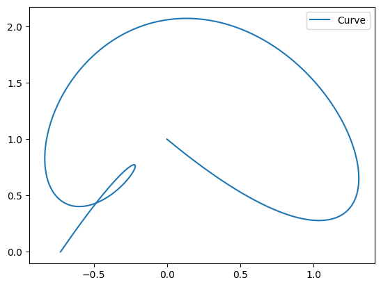
first_curve, second_curve, third_curve = curve_points.unbind(dim=1)
[70]:
plt.plot(*first_curve.unbind(dim=1), label='Curve')
plt.legend()
plt.show()
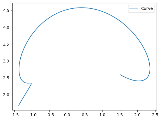
[71]:
plt.plot(*second_curve.unbind(dim=1), label='Curve')
plt.legend()
plt.show()
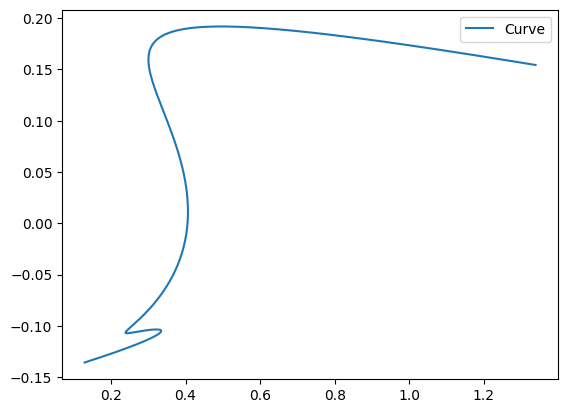
[72]:
plt.plot(*third_curve.unbind(dim=1), label='Curve')
plt.legend()
plt.show()
[ ]: