B-Spline curve plotting demo#

In this notebook we demonstrate the spatial nature of B-Spline curves - their parameters serve as control points that define the curve’s shape in space.

[10]:

import math

import matplotlib.pyplot as plt
import torch

import torchcurves.functional as tcf

Define knots#

[11]:

n_control_points = 11
degree = 3
knots = tcf.uniform_augmented_knots(n_control_points, degree)
knots

[11]:

tensor([-1.0000, -1.0000, -1.0000, -1.0000, -0.7500, -0.5000, -0.2500,  0.0000,
         0.2500,  0.5000,  0.7500,  1.0000,  1.0000,  1.0000,  1.0000])

Define control points of various shapes#

[12]:

num_curves = 3
dim = 2

t = torch.linspace(-1, 1, n_control_points)

pi = math.pi
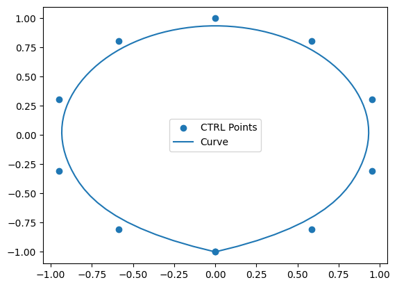
first_cp = torch.stack([torch.sin(pi * t), torch.cos(pi * t)], dim=1)
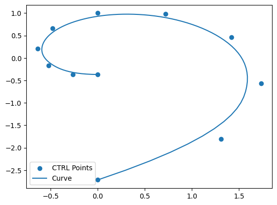
second_cp = torch.stack([torch.sin(pi * t) * t.exp(), torch.cos(pi * t) * t.exp()], dim=1)
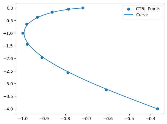
third_cp = torch.stack([t.square() + t - t.exp(), -t.square() + 2 * t - 1], dim=1)
control_points = torch.stack([first_cp, second_cp, third_cp], dim=0)
control_points.shape

[12]:

torch.Size([3, 11, 2])

Sample and draw the B-Spline curves with 100 sample points from -1 to 1#

[13]:

sample_points = torch.torch.linspace(-1, 1, 100)
spline_args = sample_points.reshape(-1, 1).expand(-1, 3)

[14]:

curve_points = tcf.bspline_curves(spline_args, control_points)
curve_points.shape

[14]:

torch.Size([100, 3, 2])

[15]:

first_curve, second_curve, third_curve = curve_points.unbind(dim=1)

[16]:

plt.scatter(*first_cp.unbind(dim=1), label='CTRL Points')
plt.plot(*first_curve.unbind(dim=1), label='Curve')
plt.legend()
plt.show()

../_images/examples_draw_bspline_10_0.png

[17]:

plt.scatter(*second_cp.unbind(dim=1), label='CTRL Points')
plt.plot(*second_curve.unbind(dim=1), label='Curve')
plt.legend()
plt.show()

../_images/examples_draw_bspline_11_0.png

[18]:

plt.scatter(*third_cp.unbind(dim=1), label='CTRL Points')
plt.plot(*third_curve.unbind(dim=1), label='Curve')
plt.legend()
plt.show()

../_images/examples_draw_bspline_12_0.png

[ ]: